Case 3 literature triangulation
This RMarkdown document demonstrates how key elements from the notebook for case study 3 in the EpiGraphDB paper can be achieved using the R package. For detailed explanations of the case study please refer to the paper or the case study notebook.
Context
The biomedical literature contains a wealth of information than far exceeds our capacity for systematic manual extraction. For this reason, there are many existing literature mining methods to extract the key concepts and content. Here we use data from SemMedDB, a well established database that provides subject-predicate-object triples from all PubMed titles and abstracts. Using a subset of this data we created MELODI-presto (https://melodi-presto.mrcieu.ac.uk/), a method to assign triples to any given biomedical query via a PubMed search and some basic enrichment, and have applied this systematically to traits represented in EpiGraphDB. This allows us to identify overlapping terms connecting any set of GWAS traits, e.g. exposure and disease outcome. From here we can attempt to triangulate causal estimates, and conversely, check the mechanisms identified from the literature against the causal evidence.
This case study goes as follows:
- For an exposure trait we identify its causal evidence against other outcome traits, then link the outcomes to diseases
- Then for an exposure-outcome pair we look for its literature evidence, and the mechanisms (as SemMed triples) identified from the literature evidence
- Finally we look into detail the mechanisms specifically related to an overlapping term and visualise these mechanisms.
library("magrittr")
library("dplyr")
#>
#> Attaching package: 'dplyr'
#> The following objects are masked from 'package:stats':
#>
#>     filter, lag
#> The following objects are masked from 'package:base':
#>
#>     intersect, setdiff, setequal, union
library("purrr")
#>
#> Attaching package: 'purrr'
#> The following object is masked from 'package:magrittr':
#>
#>     set_names
library("glue")
library("ggplot2")
library("igraph")
#>
#> Attaching package: 'igraph'
#> The following objects are masked from 'package:purrr':
#>
#>     compose, simplify
#> The following objects are masked from 'package:dplyr':
#>
#>     as_data_frame, groups, union
#> The following objects are masked from 'package:stats':
#>
#>     decompose, spectrum
#> The following object is masked from 'package:base':
#>
#>     union
library("epigraphdb")
#>
#>     EpiGraphDB v1.0 (API: https://api.epigraphdb.org)
#>
Here we set the starting trait, which we will use to explore associated disease traits.
STARTING_TRAIT <- "Sleep duration"
Get traits MR association
Given an exposure trait, find all traits with causal evidence. This method searches the causal evidence data for cases where our exposure trait has a potential casual effect on an outcome trait.
get_mr <- function(trait) {
  endpoint <- "/mr"
  params <- list(
    exposure_trait = trait,
    pval_threshold = 1e-10
  )
  mr_df <- query_epigraphdb(route = endpoint, params = params, mode = "table")
  mr_df
}

mr_df <- get_mr(STARTING_TRAIT)
mr_df %>% glimpse()
#> Rows: 1,178
#> Columns: 10
#> $ exposure.id    <chr> "ieu-a-1088", "ieu-a-1088", "ieu-a-1088", "ieu-a-1088",…
#> $ exposure.trait <chr> "Sleep duration", "Sleep duration", "Sleep duration", "…
#> $ outcome.id     <chr> "met-a-353", "met-a-307", "ieu-a-99", "ieu-a-59", "ieu-…
#> $ outcome.trait  <chr> "Cortisol", "Cholesterol", "Hip circumference", "Hip ci…
#> $ mr.b           <dbl> 0.059176931, -0.024282343, -0.288661815, 0.072874008, 0…
#> $ mr.se          <dbl> 1.385651e-03, 5.409778e-05, 5.928478e-03, 1.617032e-04,…
#> $ mr.pval        <dbl> 0, 0, 0, 0, 0, 0, 0, 0, 0, 0, 0, 0, 0, 0, 0, 0, 0, 0, 0…
#> $ mr.method      <chr> "FE IVW", "FE IVW", "FE IVW", "FE IVW", "FE IVW", "FE I…
#> $ mr.selection   <chr> "DF", "DF", "DF", "DF", "DF", "DF", "DF", "DF", "DF", "…
#> $ mr.moescore    <dbl> 1, 1, 1, 1, 1, 1, 1, 1, 1, 1, 1, 1, 1, 1, 1, 1, 1, 1, 1…
Map outcome traits to disease
For this example, we are interested in traits mapped to a disease node. To do this we utilise the mapping from GWAS trait to Disease via EFO term.
# NOTE: this block takes a bit of time, depending on the size of `mr_df` above.
#       We will not run the block here in package building,
#       but readers are encouraged to try it offline!
trait_to_disease <- function(trait) {
  endpoint <- "/ontology/gwas-efo-disease"
  params <- list(trait = trait)
  disease_df <- query_epigraphdb(route = endpoint, params = params, mode = "table")
  if (nrow(disease_df) > 0) {
    res <- disease_df %>% pull(`disease.label`)
  } else {
    res <- c()
  }
  res
}

outcome_disease_df <- mr_df %>%
  select(`outcome.trait`) %>%
  distinct() %>%
  mutate(disease = map(`outcome.trait`, trait_to_disease)) %>%
  filter(map_lgl(`disease`, function(x) !is.null(x)))
outcome_disease_df
Take one example to look for literature evidence
For the multiple exposure -> outcome relationships as reported from
the table above, here we look at the literature evidence for one pair in
detail:
- Trait X: “Sleep duration” (ieu-a-1088)
- Trait Y: “Coronary heart disease” (ieu-a-6).
The following looks for enriched triples of information (Subject-Predicate-Object) associated with our two traits. These have been derived via PubMed searches and corresponding SemMedDB data.
get_gwas_pair_literature <- function(gwas_id, assoc_gwas_id) {
  endpoint <- "/literature/gwas/pairwise"
  # NOTE in this example we blacklist to semmentic types
  params <- list(
    gwas_id = gwas_id,
    assoc_gwas_id = assoc_gwas_id,
    by_gwas_id = TRUE,
    pval_threshold = 1e-1,
    semmantic_types = "nusq",
    semmantic_types = "dsyn",
    blacklist = TRUE,
    limit = 1000
  )
  lit_df <- query_epigraphdb(route = endpoint, params = params, mode = "table")
  lit_df
}

GWAS_ID_X <- "ieu-a-1088"
GWAS_ID_Y <- "ieu-a-6"
lit_df <- get_gwas_pair_literature(GWAS_ID_X, GWAS_ID_Y)

glimpse(lit_df)
#> Rows: 1,000
#> Columns: 20
#> $ gwas.id          <chr> "ieu-a-1088", "ieu-a-1088", "ieu-a-1088", "ieu-a-1088…
#> $ gwas.trait       <chr> "Sleep duration", "Sleep duration", "Sleep duration",…
#> $ gs1.pval         <dbl> 8.663661e-06, 4.384009e-04, 7.795019e-05, 1.154660e-0…
#> $ gs1.localCount   <int> 2, 2, 2, 2, 2, 2, 2, 2, 2, 2, 2, 2, 2, 2, 2, 2, 2, 3,…
#> $ st1.name         <chr> "ADRA1D", "Hypnotics and Sedatives", "Narcotics", "Ni…
#> $ s1.id            <chr> "146:INTERACTS_WITH:C0001962", "C0020592:INTERACTS_WI…
#> $ s1.subject_id    <chr> "146", "C0020592", "C0027415", "C0068821", "C0027358"…
#> $ s1.object_id     <chr> "C0001962", "C0001962", "C0001962", "C0001962", "C000…
#> $ s1.predicate     <chr> "INTERACTS_WITH", "INTERACTS_WITH", "INTERACTS_WITH",…
#> $ st.name          <chr> "ethanol", "ethanol", "ethanol", "ethanol", "ethanol"…
#> $ st.type          <list> <"orch", "phsu">, <"orch", "phsu">, <"orch", "phsu">…
#> $ s2.id            <chr> "C0001962:COEXISTS_WITH:C0003138", "C0001962:COEXISTS…
#> $ s2.subject_id    <chr> "C0001962", "C0001962", "C0001962", "C0001962", "C000…
#> $ s2.object_id     <chr> "C0003138", "C0003138", "C0003138", "C0003138", "C000…
#> $ s2.predicate     <chr> "COEXISTS_WITH", "COEXISTS_WITH", "COEXISTS_WITH", "C…
#> $ gs2.pval         <dbl> 0.001627351, 0.001627351, 0.001627351, 0.001627351, 0…
#> $ gs2.localCount   <int> 2, 2, 2, 2, 2, 2, 2, 2, 2, 2, 2, 2, 2, 2, 2, 2, 2, 2,…
#> $ st2.name         <chr> "Antacids", "Antacids", "Antacids", "Antacids", "Anta…
#> $ assoc_gwas.id    <chr> "ieu-a-6", "ieu-a-6", "ieu-a-6", "ieu-a-6", "ieu-a-6"…
#> $ assoc_gwas.trait <chr> "Coronary heart disease", "Coronary heart disease", "…
# Predicate counts for SemMed triples for trait X
lit_df %>%
  count(`s1.predicate`) %>%
  arrange(desc(n))
#> # A tibble: 7 × 2
#>   s1.predicate           n
#>   <chr>              <int>
#> 1 INTERACTS_WITH       752
#> 2 INHIBITS              84
#> 3 STIMULATES            80
#> 4 NEG_INTERACTS_WITH    55
#> 5 COEXISTS_WITH         17
#> 6 higher_than           11
#> 7 CONVERTS_TO            1
# Predicate counts for SemMed triples for trait Y
lit_df %>%
  count(`s2.predicate`) %>%
  arrange(desc(n))
#> # A tibble: 15 × 2
#>    s2.predicate            n
#>    <chr>               <int>
#>  1 STIMULATES            179
#>  2 CAUSES                163
#>  3 TREATS                 99
#>  4 PREDISPOSES            86
#>  5 PREVENTS               79
#>  6 INHIBITS               74
#>  7 ASSOCIATED_WITH        71
#>  8 INTERACTS_WITH         71
#>  9 AFFECTS                61
#> 10 COEXISTS_WITH          61
#> 11 DISRUPTS               24
#> 12 NEG_PREVENTS           24
#> 13 higher_than             3
#> 14 NEG_ASSOCIATED_WITH     3
#> 15 AUGMENTS                2
Filter the data by predicates
Sometimes it is preferable to filter the SemMedDB data, e.g. to remove less informative Predicates, such as COEXISTS_WITH and ASSOCIATED_WITH.
# Filter out some predicates that are not informative
pred_filter <- c("COEXISTS_WITH", "ASSOCIATED_WITH")
lit_df_filter <- lit_df %>%
  filter(
    !`s1.predicate` %in% pred_filter,
    !`s2.predicate` %in% pred_filter
  )
lit_df_filter %>%
  count(`s1.predicate`) %>%
  arrange(desc(n))
#> # A tibble: 6 × 2
#>   s1.predicate           n
#>   <chr>              <int>
#> 1 INTERACTS_WITH       679
#> 2 INHIBITS              68
#> 3 STIMULATES            55
#> 4 NEG_INTERACTS_WITH    41
#> 5 higher_than           10
#> 6 CONVERTS_TO            1
lit_df_filter %>%
  count(`s2.predicate`) %>%
  arrange(desc(n))
#> # A tibble: 13 × 2
#>    s2.predicate            n
#>    <chr>               <int>
#>  1 STIMULATES            179
#>  2 CAUSES                163
#>  3 TREATS                 91
#>  4 PREDISPOSES            86
#>  5 PREVENTS               77
#>  6 INHIBITS               72
#>  7 INTERACTS_WITH         71
#>  8 AFFECTS                59
#>  9 DISRUPTS               24
#> 10 NEG_PREVENTS           24
#> 11 higher_than             3
#> 12 NEG_ASSOCIATED_WITH     3
#> 13 AUGMENTS                2
Literature results
If we explore the full table in lit_df_filter, we can see lots of
links between the two traits, pinned on specific overlapping terms.
We can summarise the SemMedDB semantic type and number of overlapping terms:
lit_counts <- lit_df_filter %>%
  count(`st.type`, `st.name`) %>%
  arrange(`st.type`, desc(`n`))
lit_counts %>% print(n = 30)
#> # A tibble: 39 × 3
#>    st.type   st.name                                  n
#>    <list>    <chr>                                <int>
#>  1 <chr [2]> ethanol                                656
#>  2 <chr [2]> Oral anticoagulants                     13
#>  3 <chr [2]> morphine                                12
#>  4 <chr [2]> Metoprolol                              10
#>  5 <chr [2]> propofol                                 4
#>  6 <chr [2]> Diazepam                                 2
#>  7 <chr [2]> Midazolam                                2
#>  8 <chr [2]> Apomorphine                              1
#>  9 <chr [2]> gamma hydroxybutyrate                    1
#> 10 <chr [2]> Luteolin                                 1
#> 11 <chr [2]> Thiopental                               1
#> 12 <chr [1]> agonists                                12
#> 13 <chr [1]> Antidepressive Agents                    8
#> 14 <chr [1]> Anti-Anxiety Agents                      4
#> 15 <chr [1]> Anesthetics                              3
#> 16 <chr [3]> leptin                                  24
#> 17 <chr [1]> Hormones                                 2
#> 18 <chr [2]> Glycoproteins                            3
#> 19 <chr [2]> Adrenergic Receptor                      2
#> 20 <chr [2]> apolipoprotein E-4                       2
#> 21 <chr [2]> PPAR gamma                               2
#> 22 <chr [2]> glutathione                              1
#> 23 <chr [4]> Somatotropin                             4
#> 24 <chr [2]> melatonin                               48
#> 25 <chr [2]> Medroxyprogesterone 17-Acetate           3
#> 26 <chr [3]> Cytochrome P450                         10
#> 27 <chr [3]> mitogen-activated protein kinase p38     4
#> 28 <chr [3]> AHSA1                                    2
#> 29 <chr [3]> AIMP2                                    2
#> 30 <chr [3]> CRK                                      2
#> # … with 9 more rows
Note, the SemMedDB semantic types have been pre-filtered to only include a subset of possibilities.
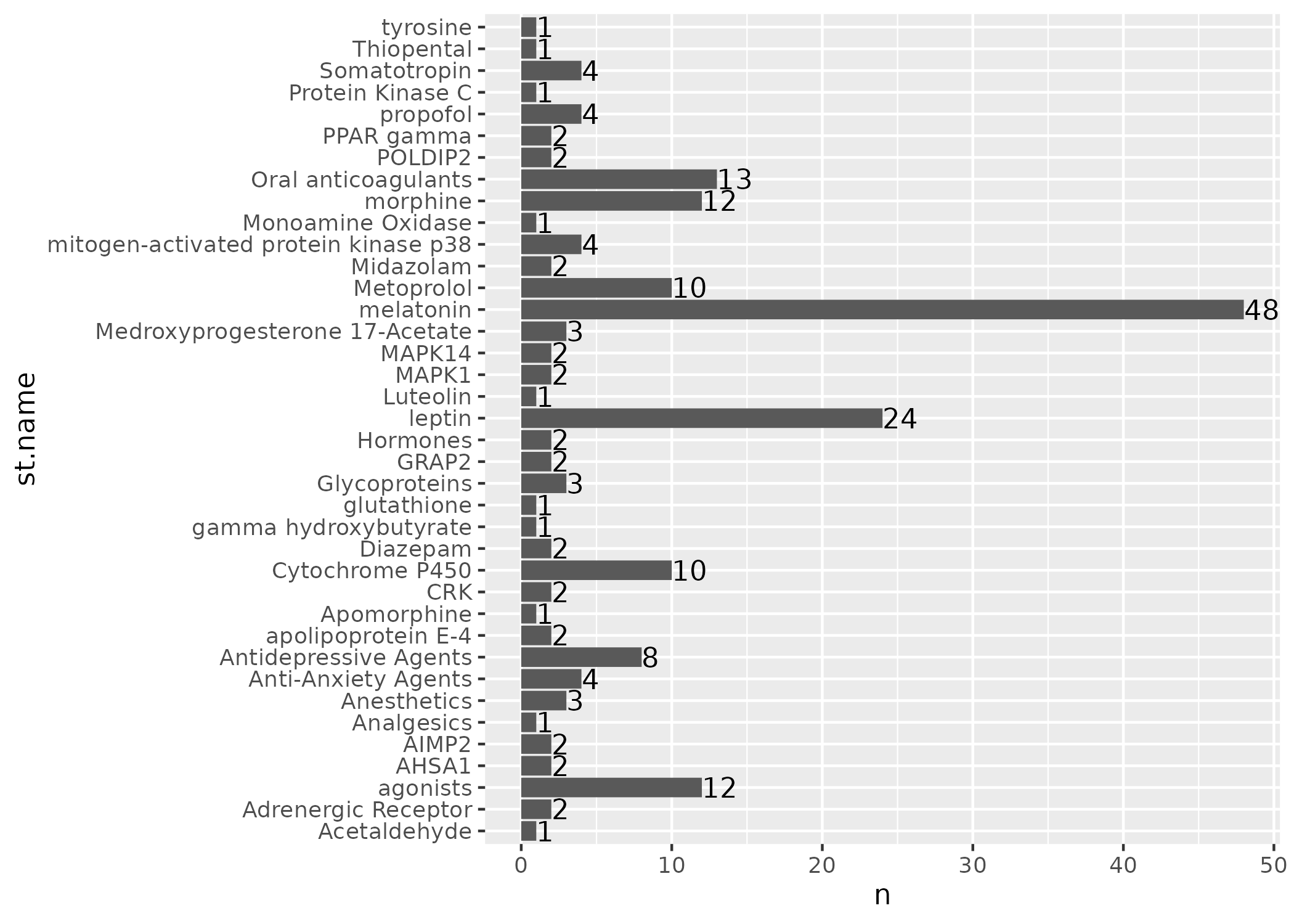
Plotting the overlapping term frequencies
We can also visualise the above table as a bar chart. In this case we will remove Ethanol as it is an outlier.
lit_counts %>%
  filter(n < 100) %>%
  {
    ggplot(.) +
      aes(x = `st.name`, y = `n`) +
      geom_col() +
      geom_text(
        aes(label = `n`),
        position = position_dodge(0.9),
        hjust = 0
      ) +
      coord_flip()
  } %>%
  ggsave(plot = ., filename="figs/case-3-term-freq.png")
#> Saving 7 x 5 in image
Look in detail at one overlapping term
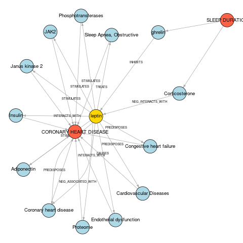
Here we look at cases where leptin is the central overlapping term.
focus_term <- "leptin"
lit_detail <- lit_df_filter %>% filter(`st.name` == focus_term)
lit_detail %>% head()
#> # A tibble: 6 × 20
#>   gwas.id    gwas.trait     gs1.pval gs1.localCount st1.name s1.id s1.subject_id
#>   <chr>      <chr>             <dbl>          <int> <chr>    <chr> <chr>
#> 1 ieu-a-1088 Sleep duration 2.48e- 6              2 Cortico… C001… C0010124
#> 2 ieu-a-1088 Sleep duration 4.62e-12              5 ghrelin  C091… C0911014
#> 3 ieu-a-1088 Sleep duration 2.48e- 6              2 Cortico… C001… C0010124
#> 4 ieu-a-1088 Sleep duration 4.62e-12              5 ghrelin  C091… C0911014
#> 5 ieu-a-1088 Sleep duration 2.48e- 6              2 Cortico… C001… C0010124
#> 6 ieu-a-1088 Sleep duration 4.62e-12              5 ghrelin  C091… C0911014
#> # … with 13 more variables: s1.object_id <chr>, s1.predicate <chr>,
#> #   st.name <chr>, st.type <list>, s2.id <chr>, s2.subject_id <chr>,
#> #   s2.object_id <chr>, s2.predicate <chr>, gs2.pval <dbl>,
#> #   gs2.localCount <int>, st2.name <chr>, assoc_gwas.id <chr>,
#> #   assoc_gwas.trait <chr>
We can create a network diagram to visualise these relationships.
lit_detail <- lit_detail %>%
  mutate_at(vars(`gwas.trait`, `assoc_gwas.trait`), stringr::str_to_upper)

# add node types: 1 - selected GWAS, 2 - traits from literature, 3 - current focus term connecting 1 and 2
nodes <- bind_rows(
  lit_detail %>% select(node = `gwas.trait`) %>% distinct() %>% mutate(node_type = 1),
  lit_detail %>% select(node = `assoc_gwas.trait`) %>% distinct() %>% mutate(node_type = 1),
  lit_detail %>% select(node = `st1.name`) %>% distinct() %>% mutate(node_type = 2),
  lit_detail %>% select(node = `st2.name`) %>% distinct() %>% mutate(node_type = 2),
  lit_detail %>% select(node = `st.name`) %>% distinct() %>% mutate(node_type = 3),
) %>% distinct()
nodes
#> # A tibble: 16 × 2
#>    node                     node_type
#>    <chr>                        <dbl>
#>  1 SLEEP DURATION                   1
#>  2 CORONARY HEART DISEASE           1
#>  3 Corticosterone                   2
#>  4 ghrelin                          2
#>  5 Sleep Apnea, Obstructive         2
#>  6 Phosphotransferases              2
#>  7 JAK2                             2
#>  8 Janus kinase 2                   2
#>  9 Insulin                          2
#> 10 Adiponectin                      2
#> 11 Coronary heart disease           2
#> 12 Proteome                         2
#> 13 Endothelial dysfunction          2
#> 14 Cardiovascular Diseases          2
#> 15 Congestive heart failure         2
#> 16 leptin                           3
edges <- bind_rows(
  # exposure -> s1 subject
  lit_detail %>%
    select(node = `gwas.trait`, assoc_node = `st1.name`) %>%
    distinct(),
  # s2 object -> outcome
  lit_detail %>%
    select(node = `st2.name`, assoc_node = `assoc_gwas.trait`) %>%
    distinct(),
  # s1 subject - s1 predicate -> s1 object
  lit_detail %>%
    select(
      node = `st1.name`, assoc_node = `st.name`,
      label = `s1.predicate`
    ) %>%
    distinct(),
  # s2 subject - s2 predicate -> s2 object
  lit_detail %>%
    select(
      node = `st.name`, assoc_node = `st2.name`,
      label = `s2.predicate`
    ) %>%
    distinct()
) %>%
  distinct()
edges
#> # A tibble: 27 × 3
#>    node                     assoc_node             label
#>    <chr>                    <chr>                  <chr>
#>  1 SLEEP DURATION           Corticosterone         <NA>
#>  2 SLEEP DURATION           ghrelin                <NA>
#>  3 Sleep Apnea, Obstructive CORONARY HEART DISEASE <NA>
#>  4 Phosphotransferases      CORONARY HEART DISEASE <NA>
#>  5 JAK2                     CORONARY HEART DISEASE <NA>
#>  6 Janus kinase 2           CORONARY HEART DISEASE <NA>
#>  7 Insulin                  CORONARY HEART DISEASE <NA>
#>  8 Adiponectin              CORONARY HEART DISEASE <NA>
#>  9 Coronary heart disease   CORONARY HEART DISEASE <NA>
#> 10 Proteome                 CORONARY HEART DISEASE <NA>
#> # … with 17 more rows
plot_network <- function(edges, nodes) {
  graph <- graph_from_data_frame(edges, directed = TRUE, vertices = nodes)
  graph$layout <- layout_with_kk

  # generate colors based on node type
  colors <- c("tomato", "lightblue", "gold")
  V(graph)$color <- colors[V(graph)$node_type]

  # Configure canvas
  default_mar <- par("mar")
  new_mar <- c(0, 0, 0, 0)
  par(mar = new_mar)

  plot.igraph(
    graph,
    vertex.size = 13,
    vertex.label.color = "black",
    vertex.label.family = "Helvetica",
    vertex.label.cex = 0.8,
    edge.arrow.size = 0.4,
    edge.label.color = "black",
    edge.label.family = "Helvetica",
    edge.label.cex = 0.5
  )
  par(mar = default_mar)
}
png(file = "figs/case-3-network-diagram.png")
plot_network(edges, nodes)
dev.off()
#> png
#>   2
Checking the source literature
We can refer back to the articles to check the text that was used to derive the SemMedDB data. This is important due to the imperfect nature of the SemRep annotation process (https://lhncbc.nlm.nih.gov/ii/tools/SemRep_SemMedDB_SKR/SemRep.html).
get_literature <- function(gwas_id, semmed_triple_id) {
  endpoint <- "/literature/gwas"
  params <- list(
    gwas_id = gwas_id,
    semmed_triple_id = semmed_triple_id,
    by_gwas_id = TRUE,
    pval_threshold = 1e-1
  )
  df <- query_epigraphdb(route = endpoint, params = params, mode = "table")
  df %>% select(`triple.id`, `triple.name`, `lit.id`)
}

pub_df <- bind_rows(
  lit_detail %>%
    select(gwas_id = `gwas.id`, semmed_triple_id = `s1.id`) %>%
    distinct(),
  lit_detail %>%
    select(gwas_id = `assoc_gwas.id`, semmed_triple_id = `s2.id`) %>%
    distinct()
) %>%
  transpose() %>%
  map_df(function(x) get_literature(x$gwas_id, x$semmed_triple_id))
pub_df
#> # A tibble: 51 × 3
#>    triple.id                            triple.name                      lit.id
#>    <chr>                                <chr>                            <chr>
#>  1 C0010124:NEG_INTERACTS_WITH:C0299583 Corticosterone NEG_INTERACTS_WI… 200515…
#>  2 C0010124:NEG_INTERACTS_WITH:C0299583 Corticosterone NEG_INTERACTS_WI… 154755…
#>  3 C0911014:INHIBITS:C0299583           ghrelin INHIBITS Leptin          216598…
#>  4 C0911014:INHIBITS:C0299583           ghrelin INHIBITS Leptin          303645…
#>  5 C0911014:INHIBITS:C0299583           ghrelin INHIBITS Leptin          224737…
#>  6 C0911014:INHIBITS:C0299583           ghrelin INHIBITS Leptin          187190…
#>  7 C0911014:INHIBITS:C0299583           ghrelin INHIBITS Leptin          199557…
#>  8 C0299583:TREATS:C0520679             Leptin|LEP TREATS Sleep Apnea, … 104496…
#>  9 C0299583:TREATS:C0520679             Leptin|LEP TREATS Sleep Apnea, … 104496…
#> 10 C0299583:STIMULATES:C0031727         Leptin STIMULATES Phosphotransf… 159272…
#> # … with 41 more rows
sessionInfo
sessionInfo()
#> R version 4.1.2 (2021-11-01)
#> Platform: x86_64-pc-linux-gnu (64-bit)
#> Running under: Ubuntu 20.04.3 LTS
#>
#> Matrix products: default
#> BLAS/LAPACK: /usr/lib/x86_64-linux-gnu/openblas-pthread/libopenblasp-r0.3.8.so
#>
#> locale:
#>  [1] LC_CTYPE=en_US.UTF-8       LC_NUMERIC=C
#>  [3] LC_TIME=en_US.UTF-8        LC_COLLATE=en_US.UTF-8
#>  [5] LC_MONETARY=en_US.UTF-8    LC_MESSAGES=en_US.UTF-8
#>  [7] LC_PAPER=en_US.UTF-8       LC_NAME=C
#>  [9] LC_ADDRESS=C               LC_TELEPHONE=C
#> [11] LC_MEASUREMENT=en_US.UTF-8 LC_IDENTIFICATION=C
#>
#> attached base packages:
#> [1] stats     graphics  grDevices utils     datasets  methods   base
#>
#> other attached packages:
#> [1] epigraphdb_0.2.3 igraph_1.2.11    ggplot2_3.3.5    glue_1.6.0
#> [5] purrr_0.3.4      dplyr_1.0.7      magrittr_2.0.1
#>
#> loaded via a namespace (and not attached):
#>  [1] pillar_1.6.4      compiler_4.1.2    tools_4.1.2       digest_0.6.29
#>  [5] jsonlite_1.7.2    evaluate_0.14     lifecycle_1.0.1   tibble_3.1.6
#>  [9] gtable_0.3.0      pkgconfig_2.0.3   rlang_0.4.12      cli_3.1.0
#> [13] DBI_1.1.2         curl_4.3.2        yaml_2.2.1        xfun_0.29
#> [17] fastmap_1.1.0     withr_2.4.3       stringr_1.4.0     httr_1.4.2
#> [21] knitr_1.37        systemfonts_1.0.3 generics_0.1.1    vctrs_0.3.8
#> [25] grid_4.1.2        tidyselect_1.1.1  R6_2.5.1          textshaping_0.3.6
#> [29] fansi_0.5.0       rmarkdown_2.11    farver_2.1.0      scales_1.1.1
#> [33] ellipsis_0.3.2    htmltools_0.5.2   assertthat_0.2.1  colorspace_2.0-2
#> [37] labeling_0.4.2    ragg_1.2.1        utf8_1.2.2        stringi_1.7.6
#> [41] munsell_0.5.0     crayon_1.4.2