Case 1 pleiotropy
This RMarkdown document demonstrates how key elements from the notebook for case study 1 in the EpiGraphDB paper can be achieved using the R package. For detailed explanations of the case study please refer to the paper or the case study notebook.
Context
Mendelian randomization (MR), a technique to evaluate the causal role of modifiable exposures on a health outcome using a set of genetic instruments, tacitly assumes that a genetic variant (e.g. SNP) is only related to an outcome of interest through an exposure (i.e. the “exclusion restriction criterion”). Horizontal pleiotropy, where a SNP is associated with multiple phenotypes independently of the exposure of interest, potentially violates this assumption delivering misleading conclusions. In contrast, vertical pleiotropy, where a SNP is associated with multiple phenotypes on the same biological pathway, does not violate this assumption.
Here, we use external evidence on biological pathways and protein-protein interactions to assess the pleiotropic profile for a genetic variant based on the genes (and proteins) with which that variant is associated. In a graph representation, we will show that:
- We have evidence of potential vertical pleiotropy when the proteins associated with a variant belong to one connected group,
- In contrast, if the proteins associated with a single variant are isolated from each other, this suggests evidence of horizontal pleiotropy.
This case study goes as follows:
- For a list of genes that we wish to assess their pleiotropic profiles (against a variant of interests), we retrieve from EpiGraphDB their mapped protein products.
- Then respectively from the evidence on shared pathway network and protein-protein interaction network, we can extract the proteins groups formed in these networks as connected communities to assess the pleiotropic profiles of the genes.
library("magrittr")
library("dplyr")
library("purrr")
library("glue")
library("igraph")
library("epigraphdb")
Here we configure the parameters used in the case study example. In this example we will look at the variant rs12720356, a SNP located in chromosome 19 that has been associated with Crohn’s disease and psoriasis.**
SNP <- "rs12720356"

GENELIST <- c("ZGLP1", "FDX1L", "MRPL4", "ICAM5", "TYK2", "GRAP2", "KRI1", "TMED1", "ICAM1")

PPI_N_INTERMEDIATE_PROTEINS <- 1
Mapping genes to proteins
The first step of the analysis is to map each of these genes to their protein product.
get_gene_protein <- function(genelist) {
  endpoint <- "/mappings/gene-to-protein"
  params <- list(
    gene_name_list = genelist %>% I()
  )
  r <- query_epigraphdb(
    route = endpoint,
    params = params,
    mode = "table",
    method = "POST"
  )
  protein_df <- r
  if (nrow(protein_df) > 0) {
    res_df <- protein_df %>%
      select(gene_name = `gene.name`, uniprot_id = `protein.uniprot_id`)
  } else {
    res_df <- tibble() %>% set_names(c("gene_name", "uniprot_id"))
  }

  res_df
}

gene_protein_df <- get_gene_protein(genelist = GENELIST)
gene_protein_df
#> # A tibble: 9 × 2
#>   gene_name uniprot_id
#>   <chr>     <chr>
#> 1 ZGLP1     P0C6A0
#> 2 FDX1L     Q6P4F2
#> 3 MRPL4     Q9BYD3
#> 4 ICAM5     Q9UMF0
#> 5 TYK2      P29597
#> 6 GRAP2     O75791
#> 7 KRI1      Q8N9T8
#> 8 TMED1     Q13445
#> 9 ICAM1     P05362
Identifying the involvement in the same biological pathways
For each protein we retrieve the pathways they are involved in.
get_protein_pathway <- function(gene_protein_df) {
  endpoint <- "/protein/in-pathway"
  params <- list(
    uniprot_id_list = gene_protein_df %>% pull(`uniprot_id`) %>% I()
  )
  df <- query_epigraphdb(route = endpoint, params = params, mode = "table", method = "POST")

  if (nrow(df) > 0) {
    res_df <- gene_protein_df %>%
      select(`uniprot_id`) %>%
      left_join(df, by = c("uniprot_id"))
  } else {
    res_df <- gene_protein_df %>%
      select(`uniprot_id`) %>%
      mutate(pathway_count = NA_integer_, pathway_reactome_id = NA_character_)
  }
  res_df <- res_df %>%
    mutate(
      pathway_count = ifelse(is.na(pathway_count), 0L, as.integer(pathway_count)),
      pathway_reactome_id = ifelse(is.na(pathway_reactome_id), c(), pathway_reactome_id)
    )

  res_df
}
pathway_df <- get_protein_pathway(gene_protein_df = gene_protein_df)
pathway_df
#> # A tibble: 9 × 3
#>   uniprot_id pathway_count pathway_reactome_id
#>   <chr>              <int> <list>
#> 1 P0C6A0                 0 <NULL>
#> 2 Q6P4F2                15 <chr [15]>
#> 3 Q9BYD3                 6 <chr [6]>
#> 4 Q9UMF0                 5 <chr [5]>
#> 5 P29597                28 <chr [28]>
#> 6 O75791                15 <chr [15]>
#> 7 Q8N9T8                 0 <NULL>
#> 8 Q13445                 0 <NULL>
#> 9 P05362                11 <chr [11]>
Now for each pair of proteins we match the pathways they have in common.
get_shared_pathway <- function(pathway_df) {
  # For the protein-pathway data
  # Get protein-protein permutations where they share pathways

  per_permutation <- function(pathway_df, permutation) {
    df <- pathway_df %>% filter(uniprot_id %in% permutation)
    primary_pathway <- pathway_df %>%
      filter(uniprot_id == permutation[1]) %>%
      pull(pathway_reactome_id) %>%
      unlist()
    assoc_pathway <- pathway_df %>%
      filter(uniprot_id == permutation[2]) %>%
      pull(pathway_reactome_id) %>%
      unlist()
    intersect(primary_pathway, assoc_pathway)
  }

  pairwise_permutations <- pathway_df %>%
    pull(`uniprot_id`) %>%
    gtools::permutations(n = length(.), r = 2, v = .)
  shared_pathway_df <- tibble(
    protein = pairwise_permutations[, 1],
    assoc_protein = pairwise_permutations[, 2]
  ) %>%
    mutate(
      shared_pathway = map2(`protein`, `assoc_protein`, function(x, y) {
        per_permutation(pathway_df = pathway_df, permutation = c(x, y))
      }),
      combination = map2_chr(`protein`, `assoc_protein`, function(x, y) {
        comb <- sort(c(x, y))
        paste(comb, collapse = ",")
      }),
      count = map_int(`shared_pathway`, function(x) na.omit(x) %>% length()),
      connected = count > 0
    )

  shared_pathway_df
}
shared_pathway_df <- get_shared_pathway(pathway_df)
n_pairs <- length(shared_pathway_df %>% filter(count > 0))
print(glue::glue("Num. shared_pathway pairs: {n_pairs}"))
#> Num. shared_pathway pairs: 6
shared_pathway_df %>% arrange(desc(count))
#> # A tibble: 72 × 6
#>    protein assoc_protein shared_pathway combination   count connected
#>    <chr>   <chr>         <list>         <chr>         <int> <lgl>
#>  1 P05362  P29597        <chr [6]>      P05362,P29597     6 TRUE
#>  2 P29597  P05362        <chr [6]>      P05362,P29597     6 TRUE
#>  3 P05362  Q9UMF0        <chr [5]>      P05362,Q9UMF0     5 TRUE
#>  4 Q9UMF0  P05362        <chr [5]>      P05362,Q9UMF0     5 TRUE
#>  5 O75791  P05362        <chr [2]>      O75791,P05362     2 TRUE
#>  6 O75791  P29597        <chr [2]>      O75791,P29597     2 TRUE
#>  7 O75791  Q9UMF0        <chr [2]>      O75791,Q9UMF0     2 TRUE
#>  8 P05362  O75791        <chr [2]>      O75791,P05362     2 TRUE
#>  9 P29597  O75791        <chr [2]>      O75791,P29597     2 TRUE
#> 10 Q9UMF0  O75791        <chr [2]>      O75791,Q9UMF0     2 TRUE
#> # … with 62 more rows
We can further query EpiGraphDB regarding the detailed pathway
information using GET /meta/nodes/Pathway/search.
get_pathway_info <- function(reactome_id) {
  endpoint <- "/meta/nodes/Pathway/search"
  params <- list(id = reactome_id)
  df <- query_epigraphdb(route = endpoint, params = params, mode = "table")
  df
}

pathway <- shared_pathway_df %>%
  pull(shared_pathway) %>%
  unlist() %>%
  unique()

pathway_info <- pathway %>% map_df(get_pathway_info)
pathway_info %>% print()
#> # A tibble: 12 × 6
#>    node._name        node.name        node._source node.id node._id node.url
#>    <chr>             <chr>            <list>       <chr>   <chr>    <chr>
#>  1 Immune System     Immune System    <chr [1]>    R-HSA-… R-HSA-1… https://rea…
#>  2 Adaptive Immune … Adaptive Immune… <chr [1]>    R-HSA-… R-HSA-1… https://rea…
#>  3 Signal Transduct… Signal Transduc… <chr [1]>    R-HSA-… R-HSA-1… https://rea…
#>  4 Interferon Signa… Interferon Sign… <chr [1]>    R-HSA-… R-HSA-9… https://rea…
#>  5 Interleukin-4 an… Interleukin-4 a… <chr [1]>    R-HSA-… R-HSA-6… https://rea…
#>  6 Interleukin-10 s… Interleukin-10 … <chr [1]>    R-HSA-… R-HSA-6… https://rea…
#>  7 Signaling by Int… Signaling by In… <chr [1]>    R-HSA-… R-HSA-4… https://rea…
#>  8 Cytokine Signali… Cytokine Signal… <chr [1]>    R-HSA-… R-HSA-1… https://rea…
#>  9 Integrin cell su… Integrin cell s… <chr [1]>    R-HSA-… R-HSA-2… https://rea…
#> 10 Immunoregulatory… Immunoregulator… <chr [1]>    R-HSA-… R-HSA-1… https://rea…
#> 11 Extracellular ma… Extracellular m… <chr [1]>    R-HSA-… R-HSA-1… https://rea…
#> 12 Disease           Disease          <chr [1]>    R-HSA-… R-HSA-1… https://rea…
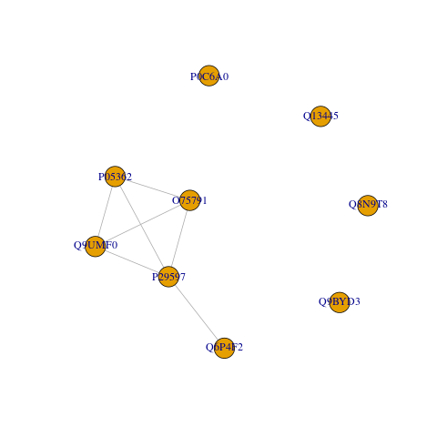
In order to extract protein groups from the shared pathways, the last step for this query is to convert the shared pathway data into a graph where
- Proteins are represented as nodes.
- And shared pathways are represented as edges.
- Then the protein groups (via shared pathways) are the connected communities in the graph.
We then count the number of nodes in each connected community and plot the graph.
protein_df_to_graph <- function(df) {
  df_connected <- df %>%
    filter(connected) %>%
    distinct(`combination`, .keep_all = TRUE)
  nodes <- df %>%
    pull(protein) %>%
    unique()
  graph <- igraph::graph_from_data_frame(
    df_connected,
    directed = FALSE, vertices = nodes
  )
  graph$layout <- igraph::layout_with_kk
  graph
}

graph_to_protein_groups <- function(graph) {
  graph %>%
    igraph::components() %>%
    igraph::groups() %>%
    tibble(group_member = .) %>%
    mutate(group_size = map_int(`group_member`, length)) %>%
    arrange(desc(group_size))
}

pathway_protein_graph <- shared_pathway_df %>% protein_df_to_graph()
pathway_protein_groups <- pathway_protein_graph %>% graph_to_protein_groups()
pathway_protein_groups %>% str()
#> tibble [5 × 2] (S3: tbl_df/tbl/data.frame)
#>  $ group_member:List of 5
#>   ..$ 1: chr [1:5] "O75791" "P05362" "P29597" "Q6P4F2" ...
#>   ..$ 2: chr "P0C6A0"
#>   ..$ 3: chr "Q13445"
#>   ..$ 4: chr "Q8N9T8"
#>   ..$ 5: chr "Q9BYD3"
#>   ..- attr(*, "dim")= int 5
#>   ..- attr(*, "dimnames")=List of 1
#>   .. ..$ : chr [1:5] "1" "2" "3" "4" ...
#>  $ group_size  : Named int [1:5] 5 1 1 1 1
#>   ..- attr(*, "names")= chr [1:5] "1" "2" "3" "4" ...
png(file = "figs/case1-pathway_protein_graph.png")
plot(pathway_protein_graph)
dev.off()
#> png
#>   2
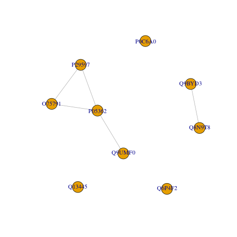
Retrieving shared protein-protein interactions
We can complement the information given by pathway ontologies with data of interactions between proteins. For each pair of proteins, we retrieve shared protein-protein interactions, either a direct interaction or an interaction where there’s one mediator protein in the middle (see parameters section).
get_ppi <- function(gene_protein_df, n_intermediate_proteins = 0) {
  endpoint <- "/protein/ppi/pairwise"
  params <- list(
    uniprot_id_list = gene_protein_df %>% pull("uniprot_id") %>% I(),
    n_intermediate_proteins = n_intermediate_proteins
  )
  df <- query_epigraphdb(
    route = endpoint,
    params = params,
    mode = "table",
    method = "POST"
  )

  if (nrow(df) > 0) {
    res_df <- gene_protein_df %>%
      select(protein = uniprot_id) %>%
      left_join(df, by = c("protein"))
  } else {
    res_df <- gene_protein_df %>%
      select(protein = uniprot_id) %>%
      mutate(assoc_protein = NA_character_, path_size = NA_integer_)
  }
  res_df
}
ppi_df <- get_ppi(gene_protein_df, n_intermediate_proteins = PPI_N_INTERMEDIATE_PROTEINS)
ppi_df
#> # A tibble: 1,686 × 3
#>    protein assoc_protein path_size
#>    <chr>   <chr>             <int>
#>  1 P0C6A0  P0C6A0                2
#>  2 P0C6A0  P0C6A0                2
#>  3 Q6P4F2  Q6P4F2                2
#>  4 Q6P4F2  Q6P4F2                2
#>  5 Q6P4F2  Q6P4F2                2
#>  6 Q6P4F2  Q6P4F2                2
#>  7 Q6P4F2  Q6P4F2                2
#>  8 Q6P4F2  Q6P4F2                2
#>  9 Q6P4F2  Q6P4F2                2
#> 10 Q6P4F2  Q6P4F2                2
#> # … with 1,676 more rows
Like in the query for pathway data, we convert and analyse these results as a graph.
get_shared_ppi <- function(ppi_df) {
  per_row <- function(ppi_df, x, y) {
    res <- ppi_df %>%
      filter(
        `protein` == x,
        `assoc_protein` == y
      ) %>%
      nrow() %>%
      `>`(0)
    res
  }

  pairwise_permutations <- ppi_df %>%
    pull(`protein`) %>%
    unique() %>%
    gtools::permutations(n = length(.), r = 2, v = .)
  shared_ppi_df <- tibble(
    protein = pairwise_permutations[, 1],
    assoc_protein = pairwise_permutations[, 2]
  ) %>%
    mutate(
      shared_ppi = map2_lgl(`protein`, `assoc_protein`, function(x, y) {
        per_row(ppi_df = ppi_df, x = x, y = y)
      }),
      combination = map2_chr(`protein`, `assoc_protein`, function(x, y) {
        comb <- sort(c(x, y))
        paste(comb, collapse = ",")
      }),
      connected = shared_ppi
    )

  shared_ppi_df
}

shared_ppi_df <- get_shared_ppi(ppi_df)
n_ppi_pairs <- shared_ppi_df %>%
  filter(shared_ppi) %>%
  nrow()
print(glue::glue("Num. shared_ppi pairs: {n_ppi_pairs}"))
#> Num. shared_ppi pairs: 10
shared_ppi_df
#> # A tibble: 72 × 5
#>    protein assoc_protein shared_ppi combination   connected
#>    <chr>   <chr>         <lgl>      <chr>         <lgl>
#>  1 O75791  P05362        TRUE       O75791,P05362 TRUE
#>  2 O75791  P0C6A0        FALSE      O75791,P0C6A0 FALSE
#>  3 O75791  P29597        TRUE       O75791,P29597 TRUE
#>  4 O75791  Q13445        FALSE      O75791,Q13445 FALSE
#>  5 O75791  Q6P4F2        FALSE      O75791,Q6P4F2 FALSE
#>  6 O75791  Q8N9T8        FALSE      O75791,Q8N9T8 FALSE
#>  7 O75791  Q9BYD3        FALSE      O75791,Q9BYD3 FALSE
#>  8 O75791  Q9UMF0        FALSE      O75791,Q9UMF0 FALSE
#>  9 P05362  O75791        TRUE       O75791,P05362 TRUE
#> 10 P05362  P0C6A0        FALSE      P05362,P0C6A0 FALSE
#> # … with 62 more rows
ppi_protein_graph <- protein_df_to_graph(shared_ppi_df)
ppi_protein_groups <- graph_to_protein_groups(ppi_protein_graph)
ppi_protein_groups %>% str()
#> tibble [5 × 2] (S3: tbl_df/tbl/data.frame)
#>  $ group_member:List of 5
#>   ..$ 1: chr [1:4] "O75791" "P05362" "P29597" "Q9UMF0"
#>   ..$ 5: chr [1:2] "Q8N9T8" "Q9BYD3"
#>   ..$ 2: chr "P0C6A0"
#>   ..$ 3: chr "Q13445"
#>   ..$ 4: chr "Q6P4F2"
#>   ..- attr(*, "dim")= int 5
#>   ..- attr(*, "dimnames")=List of 1
#>   .. ..$ : chr [1:5] "1" "5" "2" "3" ...
#>  $ group_size  : Named int [1:5] 4 2 1 1 1
#>   ..- attr(*, "names")= chr [1:5] "1" "5" "2" "3" ...
png(file = "figs/case1-ppi_protein_graph.png")
plot(ppi_protein_graph)
dev.off()
#> png
#>   2
sessionInfo
sessionInfo()
#> R version 4.1.2 (2021-11-01)
#> Platform: x86_64-pc-linux-gnu (64-bit)
#> Running under: Ubuntu 20.04.3 LTS
#>
#> Matrix products: default
#> BLAS/LAPACK: /usr/lib/x86_64-linux-gnu/openblas-pthread/libopenblasp-r0.3.8.so
#>
#> locale:
#>  [1] LC_CTYPE=en_US.UTF-8       LC_NUMERIC=C
#>  [3] LC_TIME=en_US.UTF-8        LC_COLLATE=en_US.UTF-8
#>  [5] LC_MONETARY=en_US.UTF-8    LC_MESSAGES=en_US.UTF-8
#>  [7] LC_PAPER=en_US.UTF-8       LC_NAME=C
#>  [9] LC_ADDRESS=C               LC_TELEPHONE=C
#> [11] LC_MEASUREMENT=en_US.UTF-8 LC_IDENTIFICATION=C
#>
#> attached base packages:
#> [1] stats     graphics  grDevices utils     datasets  methods   base
#>
#> other attached packages:
#> [1] epigraphdb_0.2.3 igraph_1.2.11    glue_1.6.0       purrr_0.3.4
#> [5] dplyr_1.0.7      magrittr_2.0.1
#>
#> loaded via a namespace (and not attached):
#>  [1] knitr_1.37       tidyselect_1.1.1 R6_2.5.1         rlang_0.4.12
#>  [5] fastmap_1.1.0    fansi_0.5.0      httr_1.4.2       stringr_1.4.0
#>  [9] tools_4.1.2      xfun_0.29        utf8_1.2.2       cli_3.1.0
#> [13] DBI_1.1.2        gtools_3.9.2     htmltools_0.5.2  ellipsis_0.3.2
#> [17] assertthat_0.2.1 yaml_2.2.1       digest_0.6.29    tibble_3.1.6
#> [21] lifecycle_1.0.1  crayon_1.4.2     vctrs_0.3.8      curl_4.3.2
#> [25] evaluate_0.14    rmarkdown_2.11   stringi_1.7.6    compiler_4.1.2
#> [29] pillar_1.6.4     generics_0.1.1   jsonlite_1.7.2   pkgconfig_2.0.3